1 Access site information
openair includes the function importMeta to provide
information on UK air pollution monitoring sites. There are currently
four networks that openair has access to:
- The Defra Automatic Urban and Rural Network (AURN)
- The Scottish Air Quality Network (SAQN)
- The Welsh Air Quality Network (WAQN)
- Network(s) operated by King’s College London (KCL)
These functions are described in more detail here.
The importMeta function is the first place to look to discover what
sites exist, site type (e.g. traffic, background, rural) and latitude
and longitude.
# first load openair
library(openair)

aurn <- importMeta(source = "aurn")

head(aurn)
## # A tibble: 6 x 5
## site code latitude longitude site_type
## <chr> <chr> <dbl> <dbl> <chr>
## 1 London A3 Roadside A3 51.4 -0.292 Urban Traffic
## 2 Aberdeen ABD 57.2 -2.09 Urban Background
## 3 Aberdeen Union Street Roadside ABD7 57.1 -2.11 Urban Traffic
## 4 Aberdeen Wellington Road ABD8 57.1 -2.09 Urban Traffic
## 5 Auchencorth Moss ACTH 55.8 -3.24 Rural Background
## 6 Birmingham Acocks Green AGRN 52.4 -1.83 Urban BackgroundHow many of each site type are there?
table(aurn$site_type)##
## Rural Background Suburban Background Suburban Industrial unknown unknown
## 27 8 3 4
## Urban Background Urban Industrial Urban Traffic
## 101 12 89Sometimes it is necessary to have more information on the sites such
as when they started (or stopped) measuring, the pollutants measured
and the regions in which they exist. Additional site information can
be obtained using the option all = TRUE. In the example below, we
will select sites that measure NO2 at traffic locations.
library(tidyverse)
aurn_detailed <- importMeta(source = "aurn", all = TRUE)

no2_sites <- filter(
  aurn_detailed,
  variable == "NO2",
  site_type == "Urban Traffic"
)

nrow(no2_sites)
## [1] 852 Plot sites on a map
Since openair started there have been huge developments with R and optional packages. These developments have made it much easier to manipulate and plot data e.g. with ggplot2 and the likes of dplyr. There is also now much more focus on interactive plotting, which is very useful in the context of considering air pollution sites.
In the example below the unique sites are selected from
aurn_detailed because the site repeats the number of pollutants
that are measured. Information is also collected for the map popups
and then the map is plotted.
library(leaflet)

aurn_unique <- distinct(aurn_detailed, site, .keep_all = TRUE)

# information for map markers
content <- paste(
  paste(
    aurn_unique$site,
    paste("Code:", aurn_unique$code),
    paste("Start:", aurn_unique$date_started),
    paste("End:", aurn_unique$date_ended),
    paste("Site Type:", aurn_unique$site_type),
    sep = "<br/>"
  )
)


# plot map
leaflet(aurn) %>%
  addTiles() %>%
  addMarkers(~ longitude, ~ latitude, popup = content,
             clusterOptions = markerClusterOptions())
3 Access the data
The information above should help to describe the air quality data that is easily available through openair. Access to the data is possible through a family of functions that all tend to work in a similar way. Only two pieces of information are required: the site code(s) and the year(s) of interest.
So, to import data for the industrial Port Talbot Margam site (close to a steelworks) with the site code “PT4” for 2015 to 2018, we can:
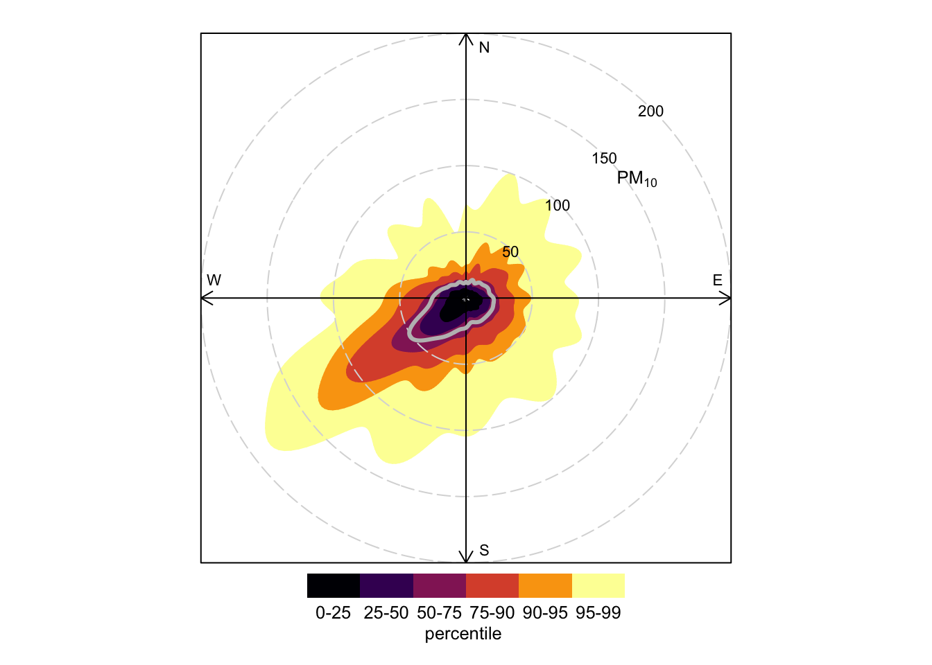
margam <- importWAQN(site = "pt4", year = 2015:2018)This data also includes estimates of wind speed and direction (ws
and wd) from the WRF model, so we can easily plot the distribution
of concentrations by wind direction. This plot indicates that the
highest PM\(_{10}\) concentrations are from the south-west i.e. the
steelworks direction. A better indication of important steelworks
combustion sources can be seen by plotting SO\(_2\).
percentileRose(margam,
               pollutant = "pm10",
               percentile = c(25, 50, 75, 90, 95, 99),
               cols = "inferno",
               smooth = TRUE
               )