openair 3.0 and 3.1: A Major New Release
The openair package has reached a significant milestone with the release of the 3.x series. Version 3.0.0 was released on CRAN on 2 April 2026, followed by 3.1.0 on 20 May 2026. Together these represent the most substantial update to openair since the original 2012 publication.
Full release notes are available on the openair news page, and a dedicated chapter in the openair book covers the changes in detail.
The big change: from lattice to ggplot2
The defining feature of openair 3.0 is that all plotting functions have been completely rewritten using ggplot2. The original package was built on lattice, which — while capable — is verbose, not particularly intuitive, and difficult to extend. The move to ggplot2 unlocks a fundamentally different workflow.
The most immediate practical benefit is that openair plots are now standard ggplot2 objects. This means you can modify them after creation using familiar ggplot2 functions:
library(openair)
library(ggplot2)

p <- timePlot(mydata, pollutant = "no2")

# Add your own annotation
p + annotate("text", x = as.POSIXct("2023-01-01"), y = 50, label = "New year")

# Apply a custom theme
p + theme_minimal()
Polar functions now use native radial coordinate systems, which removes the complex trigonometric workarounds needed under lattice and makes the underlying code more maintainable.
The transition from lattice to ggplot2 involves some breaking changes. If you have existing code that relies on lattice-specific arguments, you will need to update it. The v3 migration guide in the openair book covers what changed.
New functions
Time series filters: kzFilter() and kzaFilter()
openair 3.1 introduces Kolmogorov-Zurbenko (KZ) filters, which decompose a time series into short-term, synoptic, and long-term components. These are particularly useful for separating meteorological noise from underlying emission-driven variability.
# Decompose a NO2 time series into short/synoptic/long-term components
kzFilter(mydata, pollutant = "no2")
Flexible smoothing: WhittakerSmooth()
WhittakerSmooth() implements Whittaker-Eilers smoothing, which provides flexible smoothing and interpolation of time series and can be used to define a baseline from which anomalies can be identified. A key use case is separating local pollution increments from regional background concentrations. Compared with rolling quantile approaches, the Whittaker baseline produces a smooth, continuous curve that handles missing data naturally and avoids the abrupt step-changes that occur when observations enter or leave a rolling window.
WhittakerSmooth(mydata, pollutant = "no2", lambda = 1000)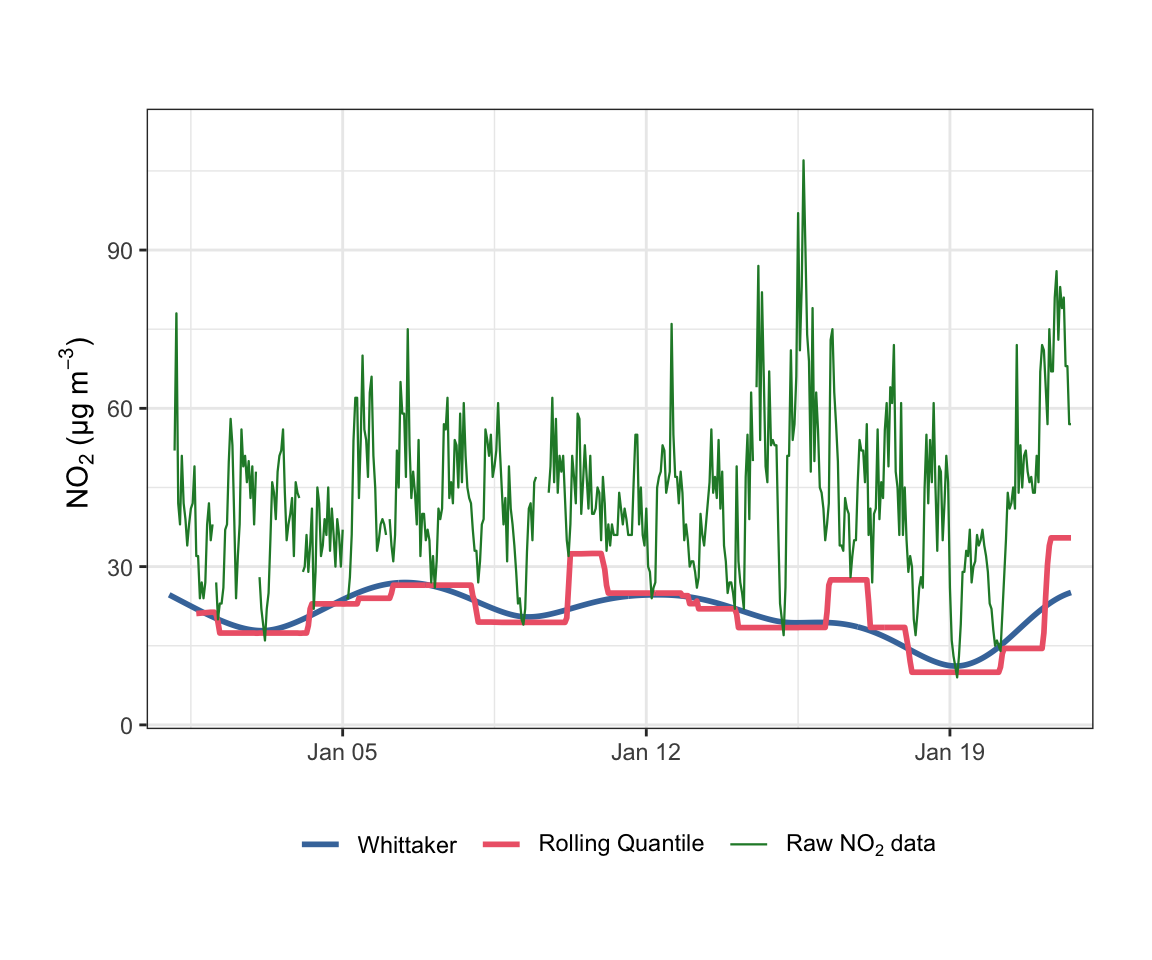
mydata. The Whittaker baseline is smooth and continuous; the rolling quantile baseline changes abruptly as observations enter or leave the window.variationPlot()
A new generalised variation plotting function that accepts arbitrary x values passed to cutData(), giving more flexibility than timeVariation() for custom temporal breakdowns.
Expanded colour and theme options
Themes
All plotting functions now accept a theme argument with five built-in options: "default", "dark", "modern", "soft", and "print". This makes it straightforward to produce consistent publication-ready or presentation-ready output.
polarPlot(mydata, pollutant = "no2", theme = "dark")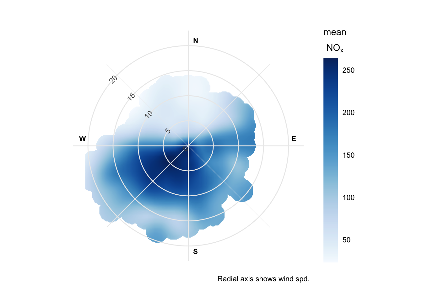
ggplot2 themeing applied to a bivariate polar plot.Colour palettes
openColours() gains several new arguments (direction, alpha, begin, end) and a set of new palettes:
- viridis family —
"rocket"and"mako"now complete the set - Paul Tol palettes —
"tol.highcontrast","tol.vibrant","tol.mediumcontrast","tol.pale","tol.dark"— perceptually uniform and accessible - Fabio Crameri palettes — a comprehensive set of scientific colour maps
A new colourOpts() function provides structured control over palette selection, and openSchemes() lists all available options.
Key breaking changes
For users upgrading from openair 2.x, the most important things to be aware of:
- Lattice arguments no longer work —
drawOpenKey()is removed;key.header/key.footerare replaced bykey.title;colis replaced bycolsthroughout - Removed functions —
summaryPlot(),calcFno2(),linearRelation()have been removed - Trajectory functions — the three projection arguments are replaced by a single
crsargument (defaulting to EPSG:4326) timeVariation()output structure — panel names and returned object structure have changed
Where old argument names are still recognised, openair will emit a warning and automatically remap them, giving you time to update your code.
Performance improvements
timeAverage() has been substantially accelerated through C++ implementation, and runRegression() uses a new algorithm that is considerably faster on large datasets. The 3.x series also requires R ≥ 4.1 and uses the native pipe (|>).
Full details for both releases are in the openair changelog. Please report any issues on GitHub.